Why Motion Profiles Matter More Than You Think

When engineers evaluate precision motion systems, the first instinct is often to examine datasheets for the biggest and boldest numbers like maximum acceleration, peak velocity, and top-end travel distances. At first glance, these numbers appear to offer a clear performance picture. But hidden beneath the surface is a much more complex story, one that, if misunderstood, can lead to performance bottlenecks, equipment damage, or even safety concerns.

It turns out that datasheet specifications are only as good as your understanding of the motion profiles behind them. Without that context, it’s possible (even likely) to build a motion specification around faulty assumptions. This blog takes a closer look at two widely used motion profiles, 2nd order and 3rd order and reveals how a disconnect between the two can derail expectations. It also examines how system mass, bus voltage, and terminology influence what can actually be achieved. Most importantly, it answers a critical question. Why does this matter?

MOTION PROFILES

Motion profiles define how a system moves from one point to another, shaping the trajectory of acceleration, velocity, and position over time. A 2nd order, or trapezoidal profile, assumes periods of constant acceleration followed by constant velocity and deceleration. It is intuitive and mathematically straightforward, and therefore commonly used by system integrators and engineers during planning stages. This kind of motion is represented in Figure 2.1, where the sharp corners of the acceleration plot make it clear that changes in force are expected to occur instantaneously.

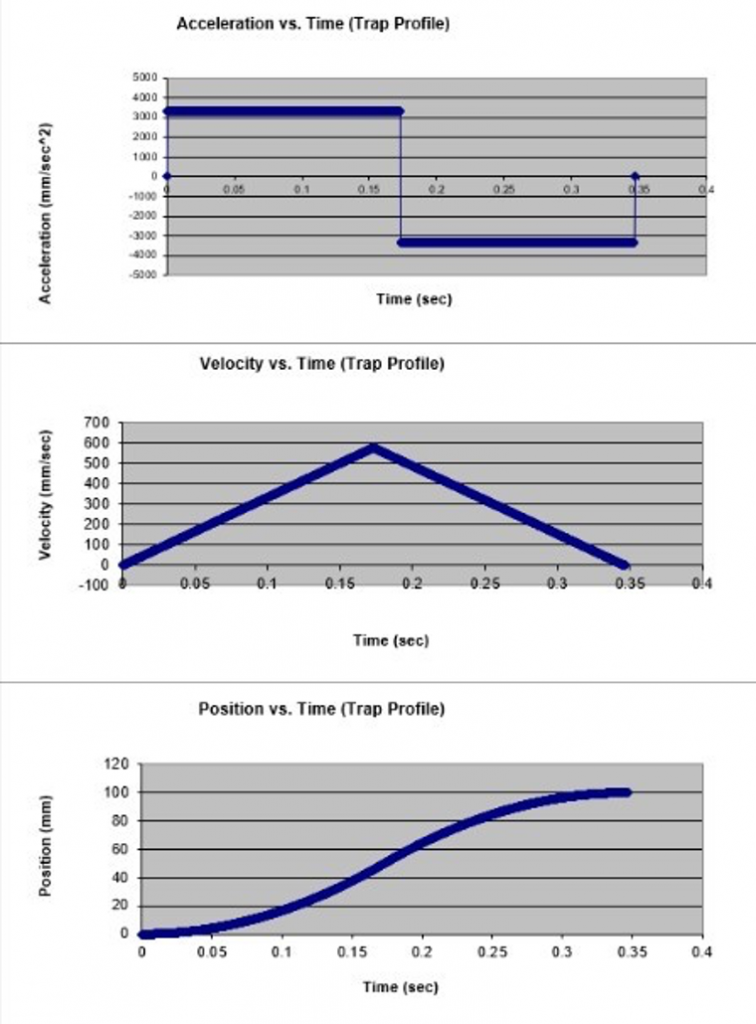
Figure 2.1. A typical 2nd order motion profile

In practice, however, motion controllers rarely use trapezoidal profiles. Instead, they implement 3rd order, or s-curve, profiles that account for jerk (the rate of change of acceleration). These profiles gradually increase and decrease acceleration to create smoother transitions, as seen in Figure 2.2. The benefits include reduced mechanical shock, quieter operation, and less wear on system components. But with those benefits comes a complication. A controller using a 3rd order profile will take longer to reach the same speed and cover more distance than a system using a 2nd order profile, unless the peak acceleration is increased significantly.

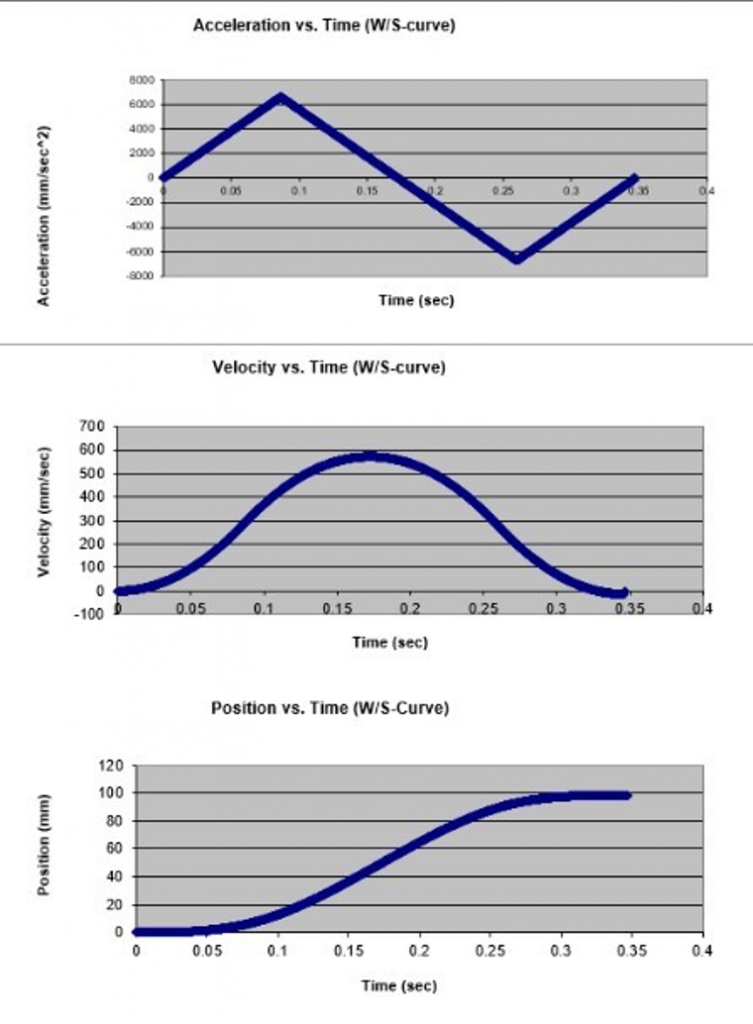
Figure 2.2 A typical 3rd order motion profile.

This gap between 2nd and 3rd order profiles often becomes a point of miscommunication between users and manufacturers. Imagine a scenario where a user needs to move a payload 100 mm using an acceleration of 3.33 m/s², with a conservative safety factor included. Their calculation, based on a 2nd order profile, estimates a move time of 350 milliseconds. However, the motion controller is working with a 3rd order profile. Because it ramps acceleration gradually, the controller will require a peak acceleration of nearly 6.66 m/s² to match the move time. Figure 3.1 visualizes this discrepancy, showing how the smoother profile must peak significantly higher to compensate for lost time during ramp-up.

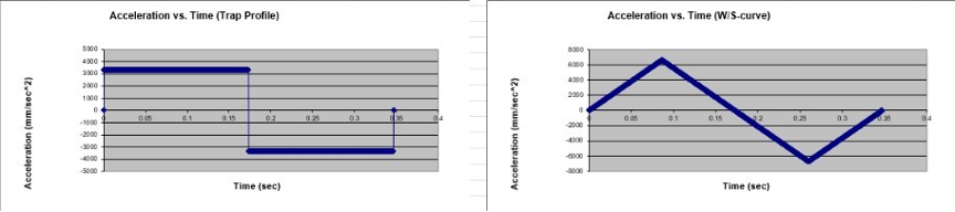
Figure 3.1. Typical 2nd and 3rd order motion profies

If the user’s payload or sensor is only rated for 5 m/s², their carefully planned motion ends up exceeding safe operating limits, even after factoring in a safety margin. The outcome could be slower-than-expected move times, diminished process efficiency, or, in extreme cases, permanent equipment damage. Worse still, if the user is providing their own motion controller and doesn’t fully understand the profile implementation, they may inadvertently command motions that exceed what the system can safely handle.

Avoiding such mismatches begins with asking clear and specific questions. When engaging a motion system provider, ambiguity is the enemy. Rather than asking whether a system can perform a move using a certain acceleration value, the user should specify the desired motion profile (trapezoidal or s-curve) and indicate the distance and time constraints explicitly. For example, asking whether a system can move 100 mm in 0.2 seconds provides a time-based constraint that avoids profile assumptions altogether. Alternatively, opening the discussion with a question about what motion the system can achieve within a specific duty cycle invites the manufacturer to define system limits clearly and on their terms.

DUTY CYCLES

Speaking of duty cycles, they are another layer of complexity that’s easy to overlook but central to performance planning. Duty cycle describes the proportion of time spent under acceleration versus the total cycle time. A high duty cycle means more sustained stress on the system, which affects how much acceleration can be applied safely. From a power dissipation standpoint, this means that even if a system can hit 10 m/s² momentarily, it may only sustain 5 m/s² at 100% duty cycle without overheating. The root mean square (RMS) acceleration, derived from the duty cycle and peak acceleration, is a more realistic benchmark for sustained motion.

MASS

Mass is another critical factor. Even when datasheets list impressive acceleration figures, they are often based on an assumed payload mass, one that might be far less than your actual load. Since acceleration is inversely proportional to mass, increasing payload reduces achievable acceleration. If you know the motor’s continuous current rating and force constant, you can calculate actual continuous force and divide it by your payload mass to get realistic acceleration numbers. These calculations rely on thermal assumptions as well. If the motor is passively cooled, allowable current (and thus force) will be lower. If the motor is actively cooled, however, performance headroom increases.

BUS VOLTAGE

Bus voltage assumptions also influence maximum velocity. A datasheet may state a rated velocity at a particular bus voltage, but your application may use a different voltage, which directly affects maximum speed. If your actual bus voltage is lower than what the manufacturer assumed, your achievable speed will be lower than advertised. A best-case scenario includes clearly stated rated speeds at known voltages, allowing engineers to work backwards from force and mass to determine whether the target motion profile is feasible.

SUMMARY

Ultimately, it’s not enough to rely on maximum velocity and acceleration values presented on a datasheet. Those figures are often theoretical best cases, not guarantees of application-level performance. The true test lies in aligning motion profile expectations with control strategy, load characteristics, thermal dynamics, and electrical constraints.

Understanding motion profiles and the assumptions behind specifications is not a luxury, it’s a necessity. In precision environments, mismatched expectations can erode system reliability, compromise throughput, and lead to costly redesigns. But with informed communication and a shared vocabulary between users and suppliers, it’s entirely possible to align real-world performance with application goals.

If you’re working on a project where motion matters (and when doesn’t it?) now is the time to go beyond the datasheet and start asking the right questions. Because the smoothest path to performance begins with a clearly defined profile.

For the detailed white paper addressing this topic, please click here – https://alioindustries.com/whitepapers/motion-profiles-and-maximum-performance-specifications/